As detailed in one of our case studies, a data centre CFD simulation project provides interesting fluid dynamics and thermal design challenges. The data hall however is not the only part of the critical infrastructure that needs heat transfer analysis. Cooling of the server and battery room requires an outdoor condenser plant. As this is exposed to elements, the environment influences its cooling performance. The goal of a condenser plant environmental CFD simulation is to tell if the designer can expect any reduction in cooling performance for certain wind speeds, directions and ambient temperatures.
How big is the simulated environment
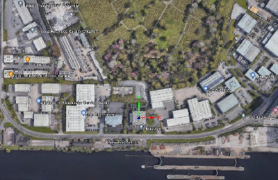
Size of the model depends on the environment where the data hall and condenser plant are. As many data centres in the UK use repurposed buildings, these sites are usually in densely built industrial parks.
We start the modelling process with locating the building in a map service. Than we copy a plan view of the area reaching a few hundred metres in radius. After inserting this plan view into our 3D CAD tool we create the model of units around the plant in a moderately detailed way. The model also contains larger individual trees and woods, especially if these are close to the plant.
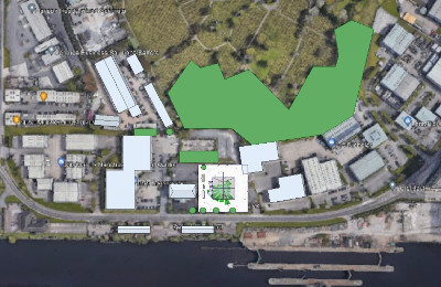
The reason is that normally there is no information available about the buildings other than the map service’s 3D view and measuring tool. The situation as far as external facade dimensions are concerned is a bit better for the data centre. But not guaranteed at all that we get highly detailed drawings.
Detailed model needed for the outdoor condenser plant
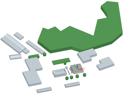
What we usually get every data of is the arrangement of the data centre site. The layout is based on a survey of the existing building. This is a good source because designers of the critical infrastructure invest a lot in getting the site dimensions right.
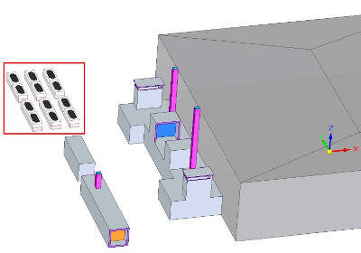
There is a third generator and an other container a bit further away from the building. Finally, we framed the subjects of our analysis in red. These are condenser units, altogether 12 of them, which release heat to the environment extracted by the air handling units in the data hall. Their operation is effected by the micro-climate other equipment on site generate in combination with macro-climate effects like ambient temperature, wind speed and direction.
Effects of the micro-climate
The most important factor of the micro-climate is air temperature. Our job is to determine the probability when these condenser units may face 35ºC or higher air temperatures at their cooling air inlet. It is a very important factor as above 35ºC inlet air, cooling performance of condensers decrease. Designers of the critical infrastructure need to know how much extra cooling capacity they need to compensate for these occasions.
There are some unfavourable scenarios regarding the micro-climate around condensers which we need to look at. One of these scenarios is the recirculating exhaust gas streams of generators into condensers. Recirculation can happen due to wind speed, direction and shape of buildings. The other could be, again due to wind speed and direction is the exhaust air of one condenser recirculating into an other one. Both of these scenarios get down to analysing what wind speeds and directions can cause such issues. We also need to calculate the probability of this happening during a calendar year is. For this we need to combine statistical weather data and fluid dynamics analyses.
Weather data for environmental CFD simulation
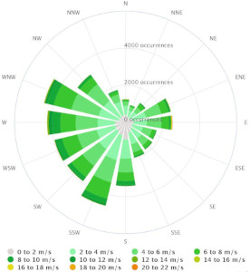
There are 16 wind directions in the rose, for each direction colours of the segment represent wind speeds. Size of the segment shows the number of occurrences that wind direction was measured during a given period. Only a few of the 16 directions could cause warm air re-circulations though. We can easily get an initial idea of which would raise some concerns.
Signs showing which wind directions to look at
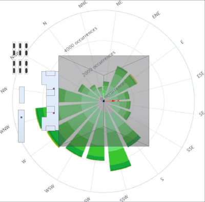
To get a feeling of what wind directions may cause trouble, we again place the wind rose on a sketch plane in the CAD system and orient it with the plant layout.
These generators only work occasionally, and when they do, out of three only two are switched on. So when working out the probability of contamination from the first two generators we will take these factors into account as well.
On the other hand a SSW wind direction for example can cause more trouble. Wind directions like this one may not only transport exhaust gases and used cooling air from the third generator, but it could also blow used cooling air from the first row of condensers into the intake of the second one. The SSW segment size shows the largest number of occurrences thus it would definitely need a closer look.
For an orientation like the above we would start from NE, where wind could cross-contaminate condensers the same way SSW or SW would. The next step would be ENE and so on until we make the whole circle back to NE. Obviously we can skip some speeds and directions if we see no sign of contamination. But for this specific example all directions need at least a check.
There is one more important parameter we need to know before starting simulations, which is air maximum daily temperature. Weather data defined this as 29.7ºC so we used that temperature as ambient wind temperature for all simulated cases.
Effects of the SSE wind direction
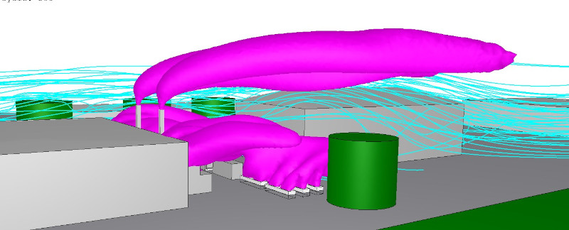
The SSE wind rose segment contains occurrences between 0m/s and 12m/s in 2m/s steps. Let’s pick 11m/s from the top tier. We also chose 5m/s from the middle and 1m/s from the low tier of wind speeds. Results below show how the purple cloud of 35ºC air changes shape with increasing wind speed. Light blue streamlines represent wind direction.
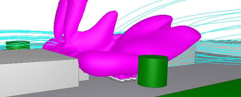
Not many signs of cross-contamination as the purple iso-surface representing the space where air temperature is 35ºC is not visible below the white coloured condensers. Let’s move on to the next wind speed.
This is getting more interesting as exhaust air plumes from generators are becoming more distinguishable. But still no obvious sign of warm air reaching below condensers. What does the highest wind speed has to show?
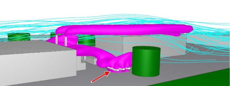
Finally the purple surface is visible underneath the condensers, so we have a positive indication for cross-contamination. When this happens, we look into the wind speeds between 5m/s and 11m/s to find out what the lowest wind speed above 5m/s is that can cause recirculation. For this specific case simulations showed that besides 11m/s also 9m/s wind speed in the SSE direction would cause higher than 35ºC temperature at condenser inlets.
CFD results tell that condenser inlet temperature for 9/s wind was 35.7ºC while it was 36.1ºC for 11m/s. Remember that ambient air (wind) temperature was 29.7ºC. Out of these two, 11m/s is more critical as it kicked inlet temperature over the limit of 35ºC by 1.1ºC.
Turning weather data and CFD results into probability
For the SSE wind direction the environmental CFD simulation showed that 9m/s and 11m/s are the wind speeds we need to take into account. To keep this example simple, we use a daily resolution of the weather data.
Weather reports tell us that there are 16 days in the year on which 9m/s wind speed was registered from the SSE direction. It also tells that there are 2 days when 11m/s speed was measured. Altogether 18 days out of 365 would mean a risk. So the probability of a contamination day due to SSE wind is 18/365=0.049 which is 4.9%. This is the first component of the probability and let’s suppose no other wind direction meant any risk.
The second is the number of days on which ambient temperature rises to, or above a level that into which mixing of the used warm air from generators or other condensers would raise condenser intakes above 35ºC.
Supposing that no other wind directions posed a contamination risk, we now know that SSE 11m/s produced the highest condenser intake temperature: 36.1ºC. This is 1.1ºC higher than critical limit of 35ºC for an ambient temperature of 29.7ºC. Logical that every temperature below 29.7 – 1.1=28.6ºC is safe. As maximum temperature rise is 6.4ºC, mixing into 25ºC ambient temperature would not cause trouble at condenser intakes. This also means that every temperature above 28.6ºC would risk a hot day.
Here comes the weather data analysis again. Throughout an average year there were 6 days on which daily maximum was at 28.7ºC or over. Probability of a hot day then is 6/365=0.0164=1.64%.
And the final probability that a day is contamination day AND a hot day = 0.049 x 0.0164=0.0008=0.08%. Pretty low I would say.
We can specify this even further by taking into account the probability of a power cut on a hot day with SSE wind direction of 9m/s or higher and the risk becomes even lower.
With these probability results at hand, critical infrastructure designers can assess risk and cost. They can decide if the outdoor condenser plant needs any additional cooling capacity.
Dr Robert Dul