A couple of years ago I had the chance to work together on a CFD service project with specialists of one of the top fan manufacturing companies in the world. Based on our discussions and running an axial fan CFD modelling benchmark project I made a short summary of the most important guidelines. This gives you a sneak peak into how professionals run CFD simulations of fans for HVAC and automotive applications.
1. Simulation of rotating motion
It is not usual to simulate the real rotating motion, later you will see why. In most of the cases however the flow field is axisymmetric to the rotation axis thus you age good to use the so called frozen rotor technique. In this method rotor blade position to stator blade is fixed .
When doing so we only need to describe the type of motion (rotation) and the angular speed coming from the electric motor RPM. The rest is done by the CFD software. We do not care about discontinuous mesh parameters and contact surfaces as we call the tools necessary to simulate real motion in SC/Tetra. The frozen rotor approach is much faster and way simpler than real life motion simulation.
What do we win with this approach? A whole bunch of time. And time is scarce in real industrial environment or in a CFD service project. The time gain is huge because these simulations are steady-state. They run fast and this is important since during a fan development a CFD guy has to run a lot of simulations.
What do we loose with this approach? A little bit of accuracy. It is so because the results could depend on the actual position of rotor and stator. Also because you cannot detect transient features like pressure variations and secondary flows.
2. Fixed volume flow rate as boundary condition
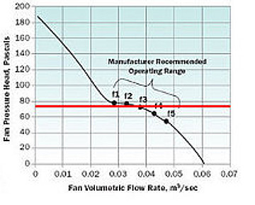
Application of a fixed volumetric flow in axial fan CFD modelling (but applies to all fan modelling really) has a straightforward reason. It comes from the fan-curve shape. Figures below show the fan-curve of an axial fan. Let’s suppose we applied the pressure difference between inlet and outlet. Say pin=75Pa is on inlet and pout=0Pa is on the outlet. If we me measured the flow rate, we would analyse our brand new fan along the red horizontal line.
That is not so good because – depending on the fan-curve – our red line may intersect with the fan-curve in more than one points. In this case you would be in trouble to tell which volume flow and which point on the fan curve is the one you are looking at for the specific 75Pa pressure drop [1].
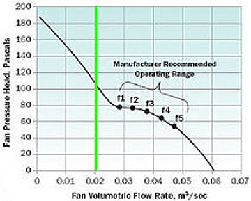
When applying fixed volume flow between inlet and outlet the green volume flow line intesects with the fan curve in only one point. As a consequence this gives only one specific pressure drop. This way you can clearly match volume flow and pressure drop pairs. For flow rate inlet CFD engineers usually apply p=0 Pa static pressure at the outlet.
Product engineers run CFD simulations across the whole fan-curve. For a given geometry (and mesh) they simulate pressure drop for a given volume flow. And here is why simulation time becomes important: you may have many volume flow points to analyse pressure loss in. Luckily in SC/Tetra this procedure can almost be fully automated.
3. Turbulence model
There is no single, universal solution for many big questions of life, and so it is with turbulence.
For example Reynolds-number and flow behaviour (whether there are any separations from blade surfaces) are the ones affecting your choice of the right turbulence model.
Depending on the actual task a good choice could be for high Re-numbers [2]:
- realizable k-ε,
- according to my experience rarely but LES (Large Eddy Simulation) is also used. The drawback of immense computational cost is significant for this type of turbulence modelling.
For low Re-numbers (in general low Re turbulence models work well for high Reynolds numbers as well):
- SST k-ω,
- AKN (Agabe-Nagano-Kondoh) k-ε,
- MPAKN k-ε.
4. Number of prismatic boundary layers
Besides turbulence modelling meshing is the other subject that still can fill many books and scientific papers.
If we just concentrate on boundary layer mesh made of prismatic elements, then the two most important parameters – thickness and number of layers – highly depend on the actual task and turbulence model. Our RnD colleagues at the fan manufacturing company for example use 6-8 layers in general. One of the references [2] mentions maximum 10 layers for high Reynolds numbers and for low Re turbulence models even 40 layers may be necessary depending on flow velocity and separation characteristics.
There are methods to estimate the thickness of the first layer but it is good practice to look into the log the solver collects while running the axial fan CFD modelling. When Y+ values do not match turbulence model requirements, you need to assess thickness of the first layer again.
5. Torque on rotor axis
One of the results professionals look at is the torque measured on the rotor axis. The CFD software calculates torque both from pressure and viscous forces. Because torque from viscous forces could reach 6-8% of the overall value you can not neglect that if you want accuracy.
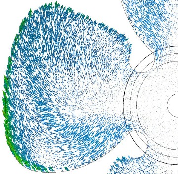
6. Shear stress on blade surfaces
Shear stress can be highlighted both as scalar (the magnitude only) and as vector on blade surfaces. The reason for calculating and analysing it is that it pretty obviously shows what is happening on the blades. If the magnitude is small, the flow separated from the surface. You can use this to highlight where blade geometry should be modified.
Dr. Robert Dul
References:
[1] Source of pictures: www.electronics-cooling.com[2] http://www.cfd-online.com/Wiki/Best_practice_guidelines_for_turbomachinery_CFD