Once the technical director of a company that engineers HVAC systems for the built environment asked me, when the time would come for the computer simulations to make traditional engineering calculations and design methods completely outdated? As far as I see it, computer simulations and engineering experience should walk hand-in-hand. More to that, I think simulations will not make fast hand calculations obsolete either. My view has been confirmed by one of our fluid dynamics motion simulation projects, in which I had to determine movements of a pipe system under external and flow induced loads. Just like years ago when we did a project for the same offshore application, we only had a few hours to do the job.
When deadline is yesterday
I received a request, whether we could simulate the motion of an underwater pipe system with water flow in it and under dynamic external load. Sure, I said, any deadline? Yesterday. Really? Really. Okay, then we find a calculation method which delivers flow induced forces by using CFD simulation. Then I combine these into a manual calculation to sum up all forces. And this hand calculation would tell if motion of the pipe is larger than the 10mm limit set by the client. Would that be okay? Yep, get on the job now.
This was how I had substituted a complex CFD simulation with a hand calculation and a simpler, faster CFD simulation. Now that I had the necessary time to perform a motion simulation on a test geometry, I am about to show you what results the hand calculation and the simulation bring to us. Are any differences between the two? Do they confirm each other’s results?
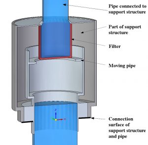
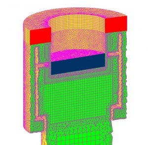
This pipe system was not only subjected to forces coming from the flow inside the pipe but also to external forces from the environment. These external forces were transferred from the support structure to the pipe through the connection surface (drawn black in the picture on the left) when the support structure moved.
Water flow within the pipe arrived through the blue coloured pipe at the bottom. This pipe was fixed to the light grey pipe head and these two together were able to move along a vertical line (in z-direction). Water flowed through the red filter and left the pipe system upwards.
Motion of the pipe meant that it was lifted from the connection plane shown by black lines.
Getting flow induced forces fast with a steady-state CFD simulation
To figure out the sum of forces that would move the pipe, we had to determine all forces (with magnitude and direction) induced by the internal water flow. For which we used a handy-dandy CFD simulation.
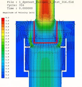
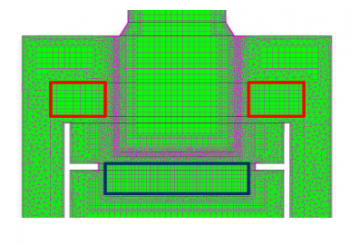
Resulting flow pattern lacks any fancy features, apart from the area around the filter. I highlighted the filter with red lines in the left picture. This filter had a 50% free area ratio, so it increased pressure loss significantly.
This was why not all the water flowed through its horizontal bottom plane. A considerable volume passed it in the gap between the lower corners of the filter and the smaller diameter collar of the pipe head. In this gap flow sped up (shown by the green colour of the scale) and entered the filter through its side near the top.
This simulation was finished quickly and SC/Tetra (the CFD code we use) calculated and collected pressure and viscosity related forces acting on the surfaces of the moving pipe. This is how they looked:
Easy to see that due to the vertical flow and the axisymmetric geometry lateral forces were minimal compared with the vertical force component. So I could neglect the lateral ones. The vertical (positive z-direction) force component of Ffz=258 N wanted to lift the moving pipe. On its own it was not enough to raise a 10ton pipe but combined with external force they could have a chance.
Complex external forces simplified
In reality external forces vary on a highly complex manner. They increase or decrease in time as the support structure moves. For this example I simplified reality quite a lot. The figure below shows the time-varying external force in orange :
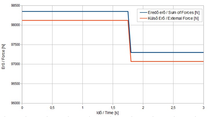
So we had a summarized force of Fsum=98350N for 1.75 seconds upwards, then an Fsum=97300N for 1.2 seconds downwards, in z-direction. Along with these there was the Fg=98000 N weight of the pipe (submerged in water) pointing down (in z-direction).
Adding up the sum of external and flow induced forces and the weight of the pipe, there was a net force of F=350N between 0 – 1.75 seconds pointing up. That could actually and truly lift up the pipe from its support platform. Between 1.8 – 3 seconds we had a net force of F=700 N pointing in negative z-direction. This pushed the pipe down towards its seat.
Force turned into distance
How can we make all this into a distance? The answer comes from Newton’s 2nd law of motion.
This law states that the net force acting on a body equals its mass times its acceleration. In short it is F=m∙a. In both the lifting and the sinking stages net F was known, because it was 350N for 1.75 seconds and 700 N for 1.2 seconds.
So I could calculate acceleration using a simple division in both stages. The acceleration was quite small: in the lifting stage it was a1=0.035m/s2, while in the sinking stage it was a2=0.0525m/s2.
To get to average velocity was a piece of cake, because it was v1=a1∙t1=0.035∙1.75=0.0613m/s for the lifting stage and v2=0.0735m/s for the sinking stage.
Distance travelled by the moving pipe came from the multiplication of average velocity and time, which gave us d1=v1∙t1=107mm for the lifting and d2=88mm for the sinking stage.
Since calculated distance in the lifting stage was 10 times bigger than the limit given by the client, I was quite sure about the answer to the initial question. Yes, the expected distance travelled would be definitely larger than the 10mm allowed maximum.
The real-life project would end here but in this example the comparison has just begun. What does the simulation tell us?
Fluid dynamics motion simulation to confirm handcalc results
I made these volumes by extruding 9 layers of mesh 14 mm thick each. These 9 layers of prism elements could stretch or shrink with no trouble at all. This property gives us the freedom to use them in various applications involving mesh deformation.
We had to take extra care when creating the mesh but after finishing that, boundary conditions could be set up in no time.
Simulation data collected automatically
It was just as easy and fast to evaluate results because SC/Tetra automatically collected motion data in a text file. This included flow induced force, travelled distance, pressure loss just to name a few. The CFD simulation software has wrote All of them as a function of time.
In pictures below I show the animation of pipe motion: on the left with velocity magnitude, on the right magnitude with velocity vectors.
It is the velocity vector animation that demonstrates how the collar of the pipe head influenced flow of water around and into the filter. Without upward motion water tended to neglect and flow past the lower third of the filter circumference. But when the pipe head was lifted, the collar forced water into this lower third of the filter as well. Due to the upward motion of the pipe head, changing flow pattern changed pressure loss of the whole system.
If a 100mm rise were allowed, the 1023 Pa increase in pressure loss as a dircet result of motion (from 9661 Pa to 10684 Pa in the highest point of the pipe travel) would also have to be taken into account in later stages of the pipe system design.
Results are very close to eachother
And the most important fact was that in the simulation the pipe moved 96mm off its support. Hand calculated result was 107mm. The difference between hand calculated and simulation results came from the fact that flow induced forces did change during pipe motion. In the fluid dynamics motion simulation flow patterns around the filter had been changing continuously. Hence the changes in induced forces.
Remember, we made only one simulation run to determine flow induced forces in the hand calculation part. We did that in the baseline position of the pipe, which was resting on its support structure before any motion could occur in reality.
For this example it really took a few hours to complete the hand calculations using a single steady-state simulation. On the other hand there were quite a few challenges with the motion simulation. Especially with creating the suitable mesh that behaved well while its size changed. I managed it no problem, but took a lot more time.
As you can see, sometimes it is quite useful to remember science subjects from secondary school, if you have just a few hours to deliver results. Also it is satisfying to know that the results from two calculation methods ended up so close to each other. No wonder at all, as even the Japanese high-tech motion simulation is based on Newton’s 2nd law.
Dr Robert Dul